QuakeR: Analyzing USGS Earthquake Data in R Markdown
Ryan J. Cooper
9/20/2022
- QuakeR:
Analyzing USGS Earthquake Data in R Markdown
- Introduction & setup
- Extract, Transform, and Load
(ETL)
- Identify USGS data sources
- Download CSV data
- Limit data analysis to earthquakes only & remove error rows
- Examine columns
- Define key constants/conversions
- Geocode terminology
- A histogram (Ogive) of earthquake event data
- Use rvest to scrape unstructure metadata
- XPath simple example
- XPath advanced example
- Examine important fields
- Exploratory Data Analysis (EDA)
- Map events on a World map projection
- Important geospatial formulas
- Exercise: Connect the dots
- Northern California Subduction zone analysis on the Gorda microplate
- Advanced map visualizations with ggmap
- References
- Appendix: Installing R
- Notes on Publishing RMarkdown
QuakeR: Analyzing USGS Earthquake Data in R Markdown
The many public and private agencies that track and analyze physical phenomena on earth provide a fascinating, never-ending source of data for R projects. In this guide, we will work with one of the amazingly rich and detailed, continually updated, readily available data sources concerning earth sciences. The data set we will explore here is provided by the U.S. Geological Survey - the premier source of data on earthquakes, coming from seismographs at a network of monitoring stations all over the world. We will explore how various R code constructs can be used to download and visualize a large data set concerning earthquake data.
Introduction & setup
R and R Markdown provide a powerful platform for accessing public data sources and developing reproducible science. Visualization capabilities in R are enhanced through the “Grammar of Graphics” as implemented through the GGPlot2 and GGForce packages. Data manipulation functions like select, mutate, and summarize are added by the dplyr package, enabling more convenient and readable R language constructs, using the pipe %>% operator. This operator can help your write intuitive syntax in R that resembles common structured query languages like SQL.
This document will not provide basic instruction in R. It is assumed that the reader has some familiarity with the R language, syntax patterns, installation, and configuration. If this is your first introduction to R, please check out the appendix to learn more about the basics of this language and installing the RStudio programming environment. The Rmd files (which this document was written in) may be downloaded from github, enabling the reader to change any portion of this document and customize the word problems to cover different applied subjects.
This project is intended for students and instructors in the field of earth sciences, GIS professionals, and anyone who is interested in using the USGS data for analysis projects in R.
Load packages
This Rmarkdown file will use several packages as defined below. This code will load the packages only of they are not already installed.
After install, these packages will be loaded into the local scope via the library functions.
#install required packages
if(!require(dplyr)) install.packages("dplyr", repos = "http://cran.us.r-project.org")
if(!require(ggplot2)) install.packages("ggplot2", repos = "http://cran.us.r-project.org")
if(!require(rvest)) install.packages("rvest", repos = "http://cran.us.r-project.org")
if(!require(stringr)) install.packages("stringr", repos = "http://cran.us.r-project.org")
if(!require(glue)) install.packages("glue", repos = "http://cran.us.r-project.org")
if(!require(maps)) install.packages("maps", repos = "http://cran.us.r-project.org")
if(!require(gridExtra)) install.packages("gridExtra", repos = "http://cran.us.r-project.org")
if(!require(gganimate)) install.packages("gganimate", repos = "http://cran.us.r-project.org")
if(!require(gifski)) install.packages("gifski", repos = "http://cran.us.r-project.org")
if(!require(geosphere)) install.packages("geosphere", repos = "http://cran.us.r-project.org")
if(!require(ggmap)) install.packages("ggmap", repos = "http://cran.us.r-project.org")
#load library into the local scope
library(dplyr)
library(ggplot2)
library(rvest)
library(stringr)
library(glue)
library(maps)
library(gridExtra)
library(gganimate)
library(geosphere)
library(gifski)
library(ggmap)
options(scipen=999)Extract, Transform, and Load (ETL)
Every R project begins with ETL. This process involves the initial set up of the project, pulling data from a dynamic data source, standardizing the data, and making it usable for your project.
Identify USGS data sources
The USGS.gov web site of the United State Geological Survey (USGS) provides a variety of scientific data sources for public use. These data sources are derived from earth sensing equipment all over the world, including earth sensing satellites, ground and sea based weather stations, and seismic monitoring facilities spanning the globe. In this guide, we will focus on how to get this data and provide visualizations from USGS sources.
Download CSV data
The first data source we will tap into is a constantly updated data source that is available as a Comma Searated Values (CSV) format. There are data feeds available in various other formats like Javascript Standard Object Notation (JSON) and Extensible Markup Language (XML), but we will use the CSV format, since it is the most basic to read and parse.
The data provides a list of all earthquakes detected in a specified time range. The rows are limited to 20,000 per query, so you have to limit the time ranges to ensure you don’t pull too many rows at the same time. Its easy to stitch the separate data sets back together using bind_rows.
The base R read.csv function is the simplest way to get this data. In this following code block we will perform 3 queries on the USGS public earthquake feed for 3 consecutive months. Note how the start date of each query is the same as the end date of the previous one.
#download a csv of earthquake data into a data frame called earthquakes_all
#earthquakes_all <- read.csv("https://earthquake.usgs.gov/earthquakes/feed/v1.0/summary/all_month.csv")
earthquakes_jul <- read.csv("https://earthquake.usgs.gov/fdsnws/event/1/query?format=csv&starttime=2022-07-01&endtime=2022-08-01")
earthquakes_aug <- read.csv("https://earthquake.usgs.gov/fdsnws/event/1/query?format=csv&starttime=2022-08-01&endtime=2022-09-01")
earthquakes_sep <- read.csv("https://earthquake.usgs.gov/fdsnws/event/1/query?format=csv&starttime=2022-09-01&endtime=2022-10-01")
#use the csv in the folder
#earthquakes_all <- read.csv("all_month-8-30.csv")
earthquakes_all <- earthquakes_jul %>% bind_rows(earthquakes_aug) %>% bind_rows(earthquakes_sep)Using the read.csv, We have downloaded a list of all earthquakes over a course of several months, so, we should have quite a few data points to work with. One might be surprised to see a list of thousands and thousands of earthquake events in a single month. Considering how infrequently we might feel an actual earthquake - It’s amazing to think that the earth is so seismically active!
We’ll now take a look at the top 10 rows to explore how the data is provided using the head function, and get a run down on the data format using the summary function.
#view some attributes of the data set
head(earthquakes_all)summary(earthquakes_all)## time latitude longitude depth
## Length:34430 Min. :-64.66 Min. :-180.0 Min. : -3.80
## Class :character 1st Qu.: 33.41 1st Qu.:-151.5 1st Qu.: 3.93
## Mode :character Median : 38.79 Median :-121.6 Median : 9.40
## Mean : 38.38 Mean :-110.1 Mean : 24.64
## 3rd Qu.: 52.92 3rd Qu.:-113.0 3rd Qu.: 19.60
## Max. : 85.43 Max. : 180.0 Max. :653.59
##
## mag magType nst gap
## Min. :-1.260 Length:34430 Min. : 0.00 Min. : 11
## 1st Qu.: 0.850 Class :character 1st Qu.: 9.00 1st Qu.: 72
## Median : 1.400 Mode :character Median : 17.00 Median :106
## Mean : 1.657 Mean : 23.73 Mean :122
## 3rd Qu.: 2.100 3rd Qu.: 30.00 3rd Qu.:160
## Max. : 7.600 Max. :444.00 Max. :360
## NA's :1 NA's :7888 NA's :7888
## dmin rms net id
## Min. : 0.000 Min. :0.0000 Length:34430 Length:34430
## 1st Qu.: 0.027 1st Qu.:0.1100 Class :character Class :character
## Median : 0.067 Median :0.1800 Mode :character Mode :character
## Mean : 0.818 Mean :0.2945
## 3rd Qu.: 0.246 3rd Qu.:0.4600
## Max. :47.586 Max. :2.2800
## NA's :13263 NA's :1
## updated place type horizontalError
## Length:34430 Length:34430 Length:34430 Min. : 0.080
## Class :character Class :character Class :character 1st Qu.: 0.280
## Mode :character Mode :character Mode :character Median : 0.520
## Mean : 2.015
## 3rd Qu.: 1.460
## Max. :99.000
## NA's :10631
## depthError magError magNst status
## Min. : 0.000 Min. :0.000 Min. : 0.00 Length:34430
## 1st Qu.: 0.450 1st Qu.:0.102 1st Qu.: 4.00 Class :character
## Median : 0.800 Median :0.155 Median : 8.00 Mode :character
## Mean : 3.195 Mean :0.254 Mean : 15.38
## 3rd Qu.: 1.818 3rd Qu.:0.232 3rd Qu.: 16.00
## Max. :16786.400 Max. :6.190 Max. :760.00
## NA's :1 NA's :8800 NA's :7925
## locationSource magSource
## Length:34430 Length:34430
## Class :character Class :character
## Mode :character Mode :character
##
##
##
## Limit data analysis to earthquakes only & remove error rows
A careful read of the type field reveals that this data set contains some event types that are not earthquakes.
earthquakes_all %>% distinct(type)For the remainder of the analysis, we will look only at earthquakes and remove explosions, quarry blasts, ice quakes, and other phenomena that are not “strictly earthquakes”.
earthquakes_all <- earthquakes_all %>% filter(type=='earthquake')
earthquakes_all <- earthquakes_all %>% filter(!is.na(mag))
earthquakes_all <- earthquakes_all %>% filter(!is.na(latitude))
earthquakes_all <- earthquakes_all %>% filter(!is.na(longitude))
earthquakes_all <- earthquakes_all %>% filter(!is.na(time))Examine columns
The earthquake data is very extensive, with 22 columns about each event - creating about 220,000 total data points.
columns_all <- colnames(earthquakes_all)
columns_all## [1] "time" "latitude" "longitude" "depth"
## [5] "mag" "magType" "nst" "gap"
## [9] "dmin" "rms" "net" "id"
## [13] "updated" "place" "type" "horizontalError"
## [17] "depthError" "magError" "magNst" "status"
## [21] "locationSource" "magSource"The data source has 22 columns of data, including location, magnitude, and many other measurements for each event. Some of these seem fairly obvious - latitude, longitude, magnitude, and time, etc. We can use the glue function from the glue package to make statements about the data and drop in R variables.
#examine the range of 4 important variables
range_lat <- range(earthquakes_all$latitude)
range_lon <- range(earthquakes_all$longitude)
range_mag <- range(earthquakes_all$mag)
range_depth <- range(earthquakes_all$depth)
glue("This data set covers a latitude range from {range_lat[1]} to {range_lat[2]} and a longuitude range from {range_lon[1]} to {range_lon[2]}. The events in this data registered between {range_mag[1]} and {range_mag[2]} on the richter scale, at depths from {range_depth[1]} to {range_depth[2]} km below sea level.")## This data set covers a latitude range from -64.6571 to 85.4314 and a longuitude range from -179.9968 to 179.9992. The events in this data registered between -1.26 and 7.6 on the richter scale, at depths from -3.8 to 653.587 km below sea level.Define key constants/conversions
earth_circum_km <- 40075
earth_diam_km <- 12742
meters_per_km <- 1000
meters_per_mile <- 1609.34As noted above, values in the latitude and longitude indicate that the data covers the majority of the planet Earth, at magnitudes that vary from hardly perceptibel events to major earthquakes. These facts raise an important question - what unit* is the depth and the magnitude? It is not clear what some of the values in the data set would be referring to unless you are have domain knowledge of USGS terminology and measures.
The USGS site does not provide any obvious link to a meta data file that defines these fields. We will explore how to get the descriptive meta data in the next section.
Geocode terminology
The term Geocode refers to the latitude and longitude pair of coordinates for any given place on earth.
 Latitude can be
understood as distance North or South from the equator. Lines of
latitude run parallel to the equator, are evenly spaced, and never touch
each other. Latitudes south of the equator are given as negative values
from 0 to -90. Latitudes north of the equator are given as positive
values from 0 to 90.
Latitude can be
understood as distance North or South from the equator. Lines of
latitude run parallel to the equator, are evenly spaced, and never touch
each other. Latitudes south of the equator are given as negative values
from 0 to -90. Latitudes north of the equator are given as positive
values from 0 to 90.
 Longitude can be
understood as distance East or West from the Prime meridian. Longitude
is generally expressed in terms of degrees to the east or west of this
line, between 0 and 180 degrees. This line was originally set as a
straight line proceeding from the north pole, through Greenwich,
England, to the South Pole. The line opposite the Prime Meridian, is
also called the anti-meridian, which runs roughly between the western
part of Alaska and the easternmost part of Russia. Lines of longitude
run perpendicular to the equator, are evenly spaced at the equator, and
converge into each other at the north and south pole. Longitudes west of
the prime meridian (0 degrees) are given as negative values from 0 to
-180. Longitudes east of the prime meridian (0 degrees) are given as
positive values from 0 to 180.
Longitude can be
understood as distance East or West from the Prime meridian. Longitude
is generally expressed in terms of degrees to the east or west of this
line, between 0 and 180 degrees. This line was originally set as a
straight line proceeding from the north pole, through Greenwich,
England, to the South Pole. The line opposite the Prime Meridian, is
also called the anti-meridian, which runs roughly between the western
part of Alaska and the easternmost part of Russia. Lines of longitude
run perpendicular to the equator, are evenly spaced at the equator, and
converge into each other at the north and south pole. Longitudes west of
the prime meridian (0 degrees) are given as negative values from 0 to
-180. Longitudes east of the prime meridian (0 degrees) are given as
positive values from 0 to 180.
A histogram (Ogive) of earthquake event data
Jumping ahead a bit, for the purpose of the following basic visualizations, I’ll reveal that magnitude is in local magnitude Richter scale units abbreviated as ML and depth is in Kilometers abbreviated as Km.
It is often a good idea to start analysis of a population with a histogram (Ogive) so we can get a rough sense of the distribution of values. There is simply no way to understand the distribution of a population data using only mean, median, and range. A histogram will start to illuminate how earthquake events are distributed by magnitude and depth.
Our first GGPlot will keep it simple - we will only provide one metric to analyze, and add a title, subtitle, and axis labels. We will add citation/attribution and more exciting customization features like colors in later charts.
Visualizing a data set in GGPlot is usually easiest when you use the dplyr package and pipe operator*. You can feed the data set into the GGPlot this way. so the syntax to do this is like this:
*In later version of R the pipe operator does not require the dplyr package to be loaded. But for this guide, we will consider it a separate package and include it.
[dataset] %>% [ggplot constructor with aesthetics parameters] + [ggplot chart type] + [plot labels]
This is perhaps the simplest way to create a ggplot and output it to the console.
earthquakes_all %>% ggplot(aes(x=mag)) +
geom_histogram() +
labs(title='Magnitude of all earthquake events',x='Magnitude (ML)',y='Count')
A histogram of events by magnitude reveals the general count of earthquakes by magnitude. This one of the simplest visualizations we can perform on the data - but it reveals quite a lot - based on this we can see that earthquakes tend to occur mostly around magnitude 1 - but there is another node around 4.25 with an increased incidence of events.
earthquakes_all %>% ggplot(aes(x=depth)) +
geom_histogram() +
labs(title='Depth of all earthquake events',x='Magnitude (ML)',y='Count')
A histogram of depth indicates a strong left skew toward shallower earthquakes with a long tail that stretches to the right indicating that the data set contains a small number of very deep earthquakes, up* to about 600 km under ground. (well, down, really!)
Use rvest to scrape unstructure metadata
We will now shift gears for a while, to address the issue of data definitions and units. Our first task in communicating data accurately is to figure out what all of the columns of data actually mean. To describe the meta data for this data set - the USGS has a dedicated web page.
The easiest thing to do would be to just go to that page and copy and paste some data definitions into the report. But let’s face it - that’s no fun, and you are not going to learn anything by doing that. So instead, we will use data scraping techniques to automatically pull the data we need from this page on the USGS site.
To parse this metadata we will use the rvest package to “harvest” data from the USGS site relating to this data source. For this task we’ll use the read_html class and several scraper methods that can walk the DOM of the USGS page using xpath, extracting the elements that are of interest to us.
This technique is very valuable when you are trying to put the pieces together from multiple data sources. It not uncommon to see systems set up like this where a dataset is a combination of structured data like CSV, JSON, or XML list, and unstructured data, like a supporting HTML page.
We won’t dive into a full tutorial on xpath here, but the code below shows how this type of syntax can be used to find elements that follow any kind of set pattern in the HTML. This image shows the HTML source code view for the web page with column definitions. Each definition seems to follow a consistent table structure:

Code of the USGS Page
XPath simple example
In this particular xpath, we are looking at the html_sections variable (the entire HTML page contents) and:
- searching for an html node using %>% html_nodes(xpath=…)
- the html node
- with the id of ‘depthError’ (//dt[@id='depthError'])
- with the id of ‘depthError’ (//dt[@id='depthError'])
- moving to the first following ‘dd’ sibling in the code
(following-sibling::dd[1])
- then stepping down to the first child
-
(/dd[1])
- then to the child
-
(/dl) of that
- and the first child
- (/dd) of that
- (/dd) of that
- finally we’re selecting just the contents of each matching tag sing the (%>% html_text) method.
This process sometimes referred to as “Walking the DOM” - Every html document has a document object model (DOM), and xpath is the map of the path we are walking through the DOM. The xpath instructs us when to stepping into an element, traverse, look up or down, etc. as we seek out a specific element or set of elements. This can be challenging process sometimes to “envision” the exact correct path - even when you are looking at the code - so it may take some trial and error to find the exact elements you are looking for.
#earthquake definitions
earthquakes_def <- read_html("https://earthquake.usgs.gov/data/comcat/index.php")
col_name <- 'depthError'
set_xpath = glue("//dt[@id='{col_name}']/following-sibling::dd[1]/dl/dd")
html_sections <- earthquakes_def %>%
html_nodes(xpath=set_xpath) %>%
html_text()
explanatory_type <- html_sections[1]
explanatory_range <- html_sections[2]
explanatory_summary <- html_sections[3]
explanatory_desc <- html_sections[4]
#after extraction we will remove newline characters using the stringr str_remove_all function
explanatory_summary <- str_remove_all(explanatory_summary, "\n")
explanatory_desc <- str_remove_all(explanatory_desc, "\n")
#and use the stringr str_squish to reduce double-spaces to make the data more readable
explanatory_summary <- str_squish(explanatory_summary)
explanatory_desc <- str_squish(explanatory_desc)
#make it a logical sentence form statement
statement <- glue("The column {col_name} is of type: {explanatory_type}. It describes the {explanatory_summary} The possible range of this variable is {explanatory_range}. This variable means: {explanatory_desc}")
statement## The column depthError is of type: Decimal. It describes the Uncertainty of reported depth of the event in kilometers. The possible range of this variable is [0, 100]. This variable means: The depth error, in km, defined as the largest projection of the three principal errors on a vertical line.Now we have a clean extract of the explanatory details for depthError. But this is just one of 22 variables - so, we are going to want to extend the code above and get the same details for every column.
Our columns_all variable has the list of columns. We will convert the above code to a function to apply the column list.
#encapsulate the function
get_explanatory <- function(col_name){
set_xpath = glue("//dt[@id='{col_name}']/following-sibling::dd[1]/dl/dd")
html_sections <- earthquakes_def %>%
html_nodes(xpath=set_xpath) %>%
html_text()
html_sections <- str_remove_all(html_sections, "\n")
html_sections <- str_squish(html_sections)
complete_list <- c(col_name,html_sections)
complete_list
}Now that we’ve encapsulated the html scan into a function, we can all this by just passing the column name were interested in.
#do a lookup
get_explanatory('depthError')## [1] "depthError"
## [2] "Decimal"
## [3] "[0, 100]"
## [4] "Uncertainty of reported depth of the event in kilometers."
## [5] "The depth error, in km, defined as the largest projection of the three principal errors on a vertical line."To further extend this concept we will use the r lapply function to “list apply” the column names into a list object. Apply functions are one of the real strengths of the R functional language. These apply functions iterate the data set much faster than while loops or for loops which are common to many languages.
#apply across all columns
defs_all <- lapply(columns_all,get_explanatory)
head(defs_all,3)## [[1]]
## [1] "time"
## [2] "Long Integer"
## [3] "Time when the event occurred. Times are reported in milliseconds since the epoch ( 1970-01-01T00:00:00.000Z), and do not include leap seconds. In certain output formats, the date is formatted for readability."
## [4] "We indicate the date and time when the earthquake initiates rupture, which is known as the \"origin\" time. Note that large earthquakes can continue rupturing for many 10's of seconds. We provide time in UTC (Coordinated Universal Time). Seismologists use UTC to avoid confusion caused by local time zones and daylight savings time. On the individual event pages, times are also provided for the time at the epicenter, and your local time based on the time your computer is set."
##
## [[2]]
## [1] "latitude"
## [2] "Decimal"
## [3] "[-90.0, 90.0]"
## [4] "Decimal degrees latitude. Negative values for southern latitudes."
## [5] "An earthquake begins to rupture at a hypocenter which is defined by a position on the surface of the earth (epicenter) and a depth below this point (focal depth). We provide the coordinates of the epicenter in units of latitude and longitude. The latitude is the number of degrees north (N) or south (S) of the equator and varies from 0 at the equator to 90 at the poles. The longitude is the number of degrees east (E) or west (W) of the prime meridian which runs through Greenwich, England. The longitude varies from 0 at Greenwich to 180 and the E or W shows the direction from Greenwich. Coordinates are given in the WGS84 reference frame. The position uncertainty of the hypocenter location varies from about 100 m horizontally and 300 meters vertically for the best located events, those in the middle of densely spaced seismograph networks, to 10s of kilometers for global events in many parts of the world."
##
## [[3]]
## [1] "longitude"
## [2] "Decimal"
## [3] "[-180.0, 180.0]"
## [4] "Decimal degrees longitude. Negative values for western longitudes."
## [5] "An earthquake begins to rupture at a hypocenter which is defined by a position on the surface of the earth (epicenter) and a depth below this point (focal depth). We provide the coordinates of the epicenter in units of latitude and longitude. The latitude is the number of degrees north (N) or south (S) of the equator and varies from 0 at the equator to 90 at the poles. The longitude is the number of degrees east (E) or west (W) of the prime meridian which runs through Greenwich, England. The longitude varies from 0 at Greenwich to 180 and the E or W shows the direction from Greenwich. Coordinates are given in the WGS84 reference frame. The position uncertainty of the hypocenter location varies from about 100 m horizontally and 300 meters vertically for the best located events, those in the middle of densely spaced seismograph networks, to 10s of kilometers for global events in many parts of the world."Now, looking at the data that has been read into the defs_all we can see there is some variance in the length of each element. Some of the nodes have 3 elements, some 4 and some 5. So this will make it a bit challenging to figure out where the data is that we need!
XPath advanced example
We will now re-create the get_explanatory function - but this time look for data using a more specific and verbose xpath pattern, and replace any missing fields, as well as removing newline characters.
#define the advanced xpath
get_explanatory2 <- function(col_name){
set_xpath_dt = glue("//dt[@id='{col_name}']/following-sibling::dd[1]/dl/dt[.='Data Type']/following-sibling::dd[1]")
html_datatype <- earthquakes_def %>%
html_nodes(xpath=set_xpath_dt) %>%
html_text()
set_xpath_dt = glue("//dt[@id='{col_name}']/following-sibling::dd[1]/dl/dt[.='Typical Values']/following-sibling::dd[1]")
html_range <- earthquakes_def %>%
html_nodes(xpath=set_xpath_dt) %>%
html_text()
set_xpath_dt = glue("//dt[@id='{col_name}']/following-sibling::dd[1]/dl/dt[.='Description']/following-sibling::dd[1]")
html_summ <- earthquakes_def %>%
html_nodes(xpath=set_xpath_dt) %>%
html_text()
set_xpath_dt = glue("//dt[@id='{col_name}']/following-sibling::dd[1]/dl/dt[.='Additional Information']/following-sibling::dd[1]")
html_desc <- earthquakes_def %>%
html_nodes(xpath=set_xpath_dt) %>%
html_text()
if(length(html_datatype)==0){html_datatype = NA}
if(length(html_range)==0){html_range = NA}
if(length(html_summ)==0){html_summ = NA}
if(length(html_desc)==0){html_desc = NA}
html_summ <- str_remove_all(html_summ, "\n")
html_desc <- str_remove_all(html_desc, "\n")
html_summ <- str_squish(html_summ)
html_desc <- str_squish(html_desc)
complete_list <- data.frame(name=col_name,type=html_datatype,range=html_range,summ=html_summ,desc=html_desc)
complete_list
}Having developed a more customized rvest function, now we can return each element as a data.frame with one labeled row and predictable, consistent columns present. If a column is not present - we will place an NA into that column.
#run the advanced function once
get_explanatory2('time')Finally we can use do.call with rbind, to bind each of the rows into a single data frame, with all the values in consistent columns.
#apply across all columns
defs_df <- do.call(rbind, lapply(columns_all, get_explanatory2))
defs_dfExamine important fields
In this section we will use some of the data set meta information we pulled to better understand the data provided in this feed.
Magnitude
defs_df %>% filter(name=='mag') %>% pull(desc)## [1] "The magnitude reported is that which the U.S. Geological Survey considers official for this earthquake, and was the best available estimate of the earthquake’s size, at the time that this page was created. Other magnitudes associated with web pages linked from here are those determined at various times following the earthquake with different types of seismic data. Although they are legitimate estimates of magnitude, the U.S. Geological Survey does not consider them to be the preferred \"official\" magnitude for the event. Earthquake magnitude is a measure of the size of an earthquake at its source. It is a logarithmic measure. At the same distance from the earthquake, the amplitude of the seismic waves from which the magnitude is determined are approximately 10 times as large during a magnitude 5 earthquake as during a magnitude 4 earthquake. The total amount of energy released by the earthquake usually goes up by a larger factor: for many commonly used magnitude types, the total energy of an average earthquake goes up by a factor of approximately 32 for each unit increase in magnitude. There are various ways that magnitude may be calculated from seismograms. Different methods are effective for different sizes of earthquakes and different distances between the earthquake source and the recording station. The various magnitude types are generally defined so as to yield magnitude values that agree to within a few-tenths of a magnitude-unit for earthquakes in a middle range of recorded-earthquake sizes, but the various magnitude-types may have values that differ by more than a magnitude-unit for very large and very small earthquakes as well as for some specific classes of seismic source. This is because earthquakes are commonly complex events that release energy over a wide range of frequencies and at varying amounts as the faulting or rupture process occurs. The various types of magnitude measure different aspects of the seismic radiation (e.g., low-frequency energy vs. high-frequency energy). The relationship among values of different magnitude types that are assigned to a particular seismic event may enable the seismologist to better understand the processes at the focus of the seismic event. The various magnitude-types are not all available at the same time for a particular earthquake. Preliminary magnitudes based on incomplete but rapidly-available data are sometimes estimated and reported. For example, the Tsunami Warning Centers will calculate a preliminary magnitude and location for an event as soon as sufficient data are available to make an estimate. In this case, time is of the essence in order to broadcast a warning if tsunami waves are likely to be generated by the event. Such preliminary magnitudes are superseded by improved estimates of magnitude as more data become available. For large earthquakes of the present era, the magnitude that is ultimately selected as the preferred magnitude for reporting to the public is commonly a moment magnitude that is based on the scalar seismic-moment of an earthquake determined by calculation of the seismic moment-tensor that best accounts for the character of the seismic waves generated by the earthquake. The scalar seismic-moment, a parameter of the seismic moment-tensor, can also be estimated via the multiplicative product rigidity of faulted rock x area of fault rupture x average fault displacement during the earthquake."Based on the above description, we can construct a generalized curve representing the relative amplitude and energy of earthquakes occurring at various magnitudes.
Relative seismic amplitude
Seismic amplitude refers to the amplitude of seismic waves from a given position relative to the epicenter (origin point) of an earthquake event. From the same location relative to the earthquake epicenter, each additional point on the Richter scale equals about 10X more amplitude than the previous point. This results in a logarithmic scale, so a 6 is 10X a 5, and a 7 is 100 x a 5, etc.
Mathematically this can be expressed as:
\(\text{Relative amplitude} = ML^10\)
Note that the y axis is not labeled, as this is a measure of relative amplitude, where you are comparing the x axis values to other values in a relative sense. The actual amplitude would depend on how far you are from the epicenter.
mags <- seq(from=1,to=9,by=.1)
relative_strengths <- mags^10
str_labels <- format(relative_strengths, scientific = TRUE, big.mark = ",")
strength_curve <- data.frame(mag=mags,relative_strength=relative_strengths)
strength_curve %>% ggplot(aes(x=mags, y=relative_strengths)) +
geom_line() +
labs(title='Magnitude vs. Amplitude of Seismic Waves',
x='Magnitude',
y='Relative Amplitude of Seismic Waves') +
scale_x_continuous(breaks=seq(from=1,to=9,by=.5)) +
scale_y_discrete(labels=str_labels)
Relative seismic energy
Seismic energy refers to the energy released by an earthquake. Each additional point on the Richter scale equals about 32X more energy than the previous point. This results in a logarithmic scale, so a 6 is 32X a 5, and a 7 is 1024 x a 5, etc.
Mathematically this can be expressed as:
\(\text{Relative energy} = ML^32\)
mags <- seq(from=1,to=9,by=.1)
relative_strengths <- (mags^32)
str_labels <- format(relative_strengths, scientific = TRUE, big.mark = ",")
energy_curve <- data.frame(mag=mags,relative_strength=relative_strengths)
energy_curve %>% ggplot(aes(x=mags, y=relative_strengths)) +
geom_line() +
labs(title='Magnitude vs. Energy of Seismic Waves',
x='Magnitude',
y='Relative Energy of Seismic Waves') +
scale_x_continuous(breaks=seq(from=1,to=9,by=.5))+
scale_y_discrete(labels=str_labels)
Depth
defs_df %>% filter(name=='depth') %>% pull(desc)## [1] "The depth where the earthquake begins to rupture. This depth may be relative to the WGS84 geoid, mean sea-level, or the average elevation of the seismic stations which provided arrival-time data for the earthquake location. The choice of reference depth is dependent on the method used to locate the earthquake, which varies by seismic network. Since ComCat includes data from many different seismic networks, the process for determining the depth is different for different events. The depth is the least-constrained parameter in the earthquake location, and the error bars are generally larger than the variation due to different depth determination methods. Sometimes when depth is poorly constrained by available seismic data, the location program will set the depth at a fixed value. For example, 33 km is often used as a default depth for earthquakes determined to be shallow, but whose depth is not satisfactorily determined by the data, whereas default depths of 5 or 10 km are often used in mid-continental areas and on mid-ocean ridges since earthquakes in these areas are usually shallower than 33 km."Combining data and meta information
Now we have a nice structure table of column information, plus a table with the actual data we are analyzing. We could use the meta information in our report, such as to display a statement explaining the definition of magnitude below the title. The subtitle explaining magnitude comes directly from the meta data we pulled using rvest. Additional detailed explanation of the variable can be added for clarity.
Citation Generator function
Since this is a scientific report, we should be very thorough and consistent in how we cite the data sources. It’s a good idea to set up a citation generator at the beginning of your project. Having developed R documents that are hundreds of pages long, and involved dozens of sources - It’s my experience that a citation function can save a huge amount of time. This function will help generate an numbered list of MLA citations for each data source in the project. This feature will help keep track of the bibliographical data we need to place into the end of our report, and ensure that as you insert new elements in the middle of your report, that it will re-sequence the numbering of each item accurately for your readers.
#create a citation generator function
cite_source <- function(cite_n,author,article,publisher,pubdate,url,accessdate){
str_cite_complete <- glue('{cite_n}. *{author}*, "{article}", *{publisher}*, {pubdate}, {url}, Accessed: {accessdate}')
str_cite_caption <- glue('{publisher}: {article} [{cite_n}]')
str_cite <- data.frame(caption=str_cite_caption,
complete=str_cite_complete)
str_cite
}
#start the citations table and counter for the references section
cite_n <- 0
all_citations <- data.frame()The next few plots will use the same citation, so we will just run the citation function once here, then re-use the same output in several plots. WE will also place the same citation into a data frame containing all citations, which we will use in the References section below.
#generate a citation
cite_n <- 1
citation <- cite_source(cite_n,"U.S. Geological Survey","ANSS Comprehensive Earthquake Catalog","USG",as.Date(Sys.Date()),"https://earthquake.usgs.gov/earthquakes/feed/v1.0/csv.php",as.Date(Sys.Date()))
all_citations <- all_citations %>% bind_rows(citation)Having dealt with all the technicalities of generating usable data, it’s time to get down to the science!
Exploratory Data Analysis (EDA)
We will start our EDA by using GGPlot to visualize the data set. Recall that the data contains over 200,000 observations - so any plots we create that map directly to event rows in our data set, would have hundreds of thousands of data points. This volume of data can be overkill for many visualizations - and in many cases, the data should be processed and simplified to make it more suitable for visualization; However, for a complex data analysis project, it’s often useful to see visualizations of the unprocessed data we are working with before we summarize, group, or otherwise transform the data. This approach will ensure that the viewer has a clear sense of each step in which data goes from its original “columns and rows” form, to a scientific visualization. Creating reproducible science through code is a powerful tool, but if there are too many algebraic transformations between raw data and end product, its easy to lose the train of thought.
Dot Plot of Magnitude vs. Depth data
We will start our EDA section with some more meaningful scientific plots. To increase the visual impact of these plots, we will start by applying color to the plot points. To improve their scientific validity, we must add captions at the bottom to ensure the data sources are clearly identified.
In the code below, we introduce Colour aesthetic mapped to depth, and the scale_colour_viridis_c chart setting object - this will give the dot plot a color on each point, and ensure the color is as obvious as possible by using a color scale called “Plasma” which ranges from a dark indigo, to red, to yellow.
Since the earthquakes occur underground, we will also set the y-axis depth as a negative value - that’s more intuitive on a chart - you can see deeper earthquakes lower, and shallower ones closer to the top.
#pull the summary for the mag and depth fields
mag_summary <- defs_df %>% filter(name=='mag') %>% pull(summ)
depth_summary <- defs_df %>% filter(name=='depth') %>% pull(summ)
#filter teh data to only the rows with both depth and mag
events_mag_depth <- earthquakes_all %>% filter(!is.na(mag)&!is.na(depth))
#create the depth-magnitude dot plot
events_mag_depth %>% ggplot(aes(x=mag, y=-depth, colour=depth)) +
geom_point() +
scale_colour_viridis_c(option = "plasma") +
labs(
title='Magnitude / Depth of All Earthquakes',
x='Magnitude (ML)',
y='Depth (Km)',
caption=paste('Source:',citation$caption))
mag_summary## [1] "The magnitude for the event. See also magType."depth_summary## [1] "Depth of the event in kilometers."Dot Plot of Magnitude with Error Bars
GGplot offers many enhancements that can be applied to the data to take advantage of other scientific measurements. One such measure is the magnitude error. The magnitude given in this data is subject to some measurement error, which varies somewhat based on the proximity of sensing equipment to the seismic event. The geom_errorbar provides a convenient way to visualize the estimated range of error that each magnitude measurement may be subject to. A plot of recent significant earthquakes over 5.0 magnitude could benefit from an error bar to understand the most likely range of magnitude values that that each event falls into.
In this visualization, we introduce the filter and slice features of dplyr. This will filter out any values that don’t have both mag and magError readings, and where the magnitude is OVER 5 ML. It will then take only the first 20 observations. Since the list is sorted by date, this means its the most recent 20 events.
#pull the summary for the mag and depth fields
mag_summary <- defs_df %>% filter(name=='mag') %>% pull(summ)
#filter the data to only the first 20 rows with both mag & magError, which are over 5 mag
events_mag_recent <- earthquakes_all %>% filter(!is.na(mag) & !is.na(magError) & mag >5) %>% slice(1:20)
#create the dot plot
events_mag_recent %>% ggplot(aes(x=time, y=mag, ymin=mag-magError, ymax=mag+magError, label=place)) +
geom_point() +
geom_errorbar() +
geom_label(aes(y=mag+.25)) + #use aes to move the labels up a little on the y axis
scale_colour_viridis_c(option = "plasma") +
labs(
title='Last 30 5+ Magnitude Events with Error Bars',
subtitle=mag_summary,
x='Time & Place',
y='Magnitude',
caption=paste('Source:',citation$caption)) +
theme(axis.text.x = element_text(angle = 90, hjust=1)) + #turn the date axis labels sideways
facet_wrap(~as.Date(time), scales = "free_x") #break it into x charts, one for each day in the data
mag_summary## [1] "The magnitude for the event. See also magType."depth_summary## [1] "Depth of the event in kilometers."Summary of Average Magnitude by Date
Another important scientific visualization in GGplot is the box plot or box and whisker plot as it is often called.
#pull the summary for the mag and depth fields
mag_summary <- defs_df %>% filter(name=='mag') %>% pull(summ)
events_mag_date <- earthquakes_all
events_mag_date <- events_mag_date %>% mutate(datetime=as.POSIXct(str_replace(str_replace(time,'T',' '),'Z',' '), format="%Y-%m-%d %H:%M:%S", tz="UTC"))
events_mag_date <- events_mag_date %>% mutate(date_only=as.POSIXct(str_replace(str_replace(time,'T',' '),'Z',' '), format="%Y-%m-%d", tz="UTC"))
events_mag_date <- events_mag_date %>% mutate(month_only=lubridate::month(date_only, label = TRUE))
#create the dot plot
events_mag_date %>%
ggplot(aes(x=month_only, y=mag)) +
geom_boxplot() +
scale_colour_viridis_c(option = "plasma") +
labs(
title='Boxplot of Magnitude by Month ',
subtitle="(Line = Median / Box = Interquartile Range / Whiskers = Largest Value <= 1.5*IQR / Points = Outliers)",
x='Month',
y='Magnitude',
caption=paste('Source:',citation$caption)) +
theme(axis.text.x = element_text(angle = 90, hjust=1)) 
mag_summary## [1] "The magnitude for the event. See also magType."depth_summary## [1] "Depth of the event in kilometers."Summary of Mean Magnitude by Date
Going a little further, we will now use the dplyr functions like group_by and summarize to “bake the data” into more palatable units. In this example, were going to summarize the mean magnitude for each day.
#pull the summary for the mag field
mag_summary <- defs_df %>% filter(name=='mag') %>% pull(summ)
#summarize the mag data by date
events_mag_date <- earthquakes_all %>%
filter(!is.na(depth)) %>%
group_by(date=as.Date(time)) %>%
summarize(mean_magnitude = mean(mag))
#create the plot
events_mag_date %>% ggplot(aes(x=date, y=mean_magnitude, fill=mean_magnitude)) + geom_col() + labs(title='Average Daily Magnitude of All U.S. Earthquakes',subtitle=mag_summary,caption=paste('Source:',citation$caption),
x='Date',
y='Mean Magnitude (ML)')
Summary of Mean Depth by Date
We can change the target of the group_by to the depth variable and re-use the above syntax. In this example, were going to summarize the mean depth for each day instead of magnitude.
mag_desc <- defs_df %>% filter(name=='depth') %>% pull(desc)
events_depth_date<- earthquakes_all %>% filter(!is.na(depth)) %>% group_by(date=as.Date(time)) %>% summarize(mean_depth = mean(depth))
events_depth_date %>%
ggplot(aes(x=date, y=mean_depth, fill=mean_depth)) +
geom_col() +
labs(title='Average Daily Depth of All Earthquakes',subtitle=mag_desc,
x='Date',
y='Mean Depth (Km)')
Map events on a World map projection
Since geological data is all about the earth, we will now shift gears to see how we can visualize this data using the latitude and longitude coordinates provided in conjunction with some world maps.
#generate a world map
#pull the summary for the mag and depth fields
mag_summary <- defs_df %>% filter(name=='mag') %>% pull(summ)
depth_summary <- defs_df %>% filter(name=='depth') %>% pull(summ)
#filter the data to only the rows with both depth and mag
events_mag_depth <- earthquakes_all %>% filter(!is.na(mag)&!is.na(depth))
#get teh maximum magnitude event in this data set
max_mag <- max(events_mag_depth$mag)
#divide by 3 to reduce point size proportionally
max_point_size <- max_mag/3
#get teh map data to draw the countries of the world
world_info <- map_data("world")
#copy data into a mapdata data set
mapdata <- earthquakes_all
#mutate the military formatted time field to a time in the R data type
mapdata <- mapdata %>% mutate(datetime=as.POSIXct(str_replace(str_replace(time,'T',' '),'Z',' '), format="%Y-%m-%d %H:%M:%S", tz="UTC"))
mapdata <- mapdata %>% mutate(date_only=as.POSIXct(str_replace(str_replace(time,'T',' '),'Z',' '), format="%Y-%m-%d", tz="UTC"))
#generate the map
wmap_all <- ggplot(data = world_info, mapping = aes(x = long, y = lat, group = group)) +
geom_polygon(color = "black", fill = "white") +
geom_point(data = mapdata,
alpha=.7,
mapping = aes(size = mag,
x = longitude,
y = latitude,
colour = depth,
group= date_only)) +
coord_quickmap() +
scale_size(range = c(.1, max_point_size)) +
scale_colour_viridis_c(option = "plasma") +
labs(title = paste("All Earthquake Events - Geographic Distribution"),
caption = paste("Data source:",citation$caption),
x="Longitude",
y="Latitude",
colour="Depth (Km)",
size="Magnitude (ML)")
#render
wmap_all
Save a map graphic
To save a map instead of outputting it to R directly, you can use the ggsave feature, feeding in the plot object you created. In many cases it will result in better quality imagery in your report.
#save teh last generated wmap_all graphic
ggsave("worldmap.png",plot = wmap_all,width=10,height=8)
#You can also use simple syntax *\!\[description\]\(path\)* to include the graphic in your report.
#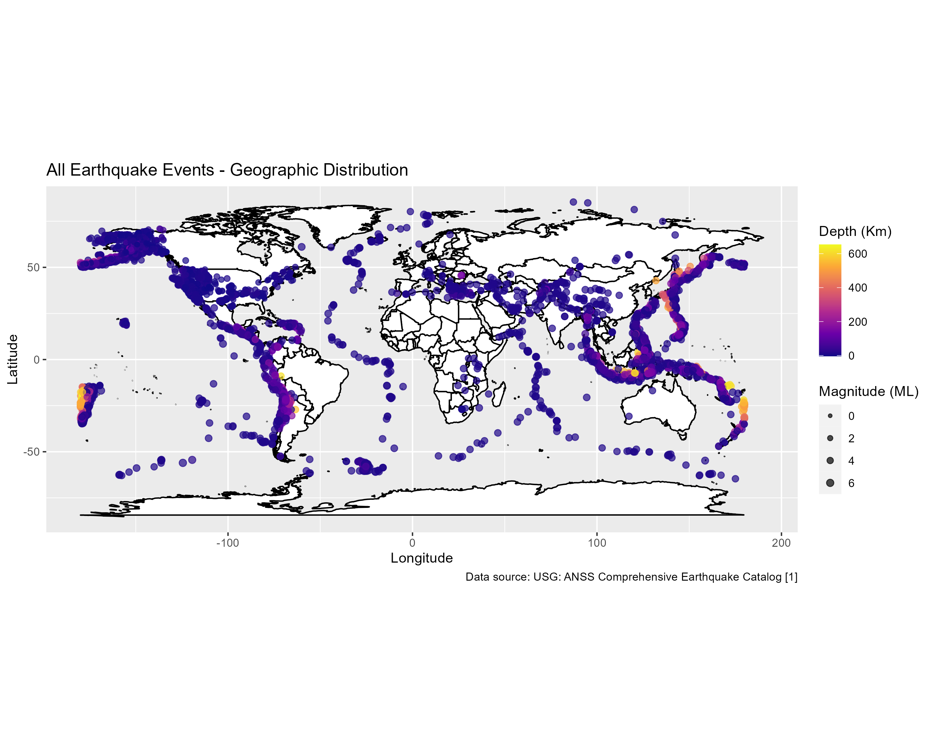This is a great start, but it’s an overwhelming amount of data to show on one map. With thousands of earthquakes, this may be more data than we really need to see all at once. We will now examine how to build a function that will produce a usable map for a more limited time frame, based on a date parameter we will pass in.
Build a reusable Map function
We will now encapsulate the quake map into a function to instead show us just one day of quakes. This will require a target date argument to be passed in for the date we want to see.
getquakemap <- function(target_date){
#get some definition data from our defs data set
mag_summary <- defs_df %>% filter(name=='mag') %>% pull(summ)
depth_summary <- defs_df %>% filter(name=='depth') %>% pull(summ)
#filter the data to only the rows with both depth and mag
events_mag_depth <- earthquakes_all %>% filter(!is.na(mag)&!is.na(depth)) %>% filter(as.Date(time) == as.Date(target_date))
#get thw maximum magnitude event in this data set
max_mag <- max(events_mag_depth$mag)
#divide by 3 to reduce point size proportionally
max_point_size <- max_mag/3
#load the outlines of continents
world_info <- map_data("world")
#copy the events mag depth table into a table called mapdata
mapdata <- events_mag_depth
#mutate the military formatted time field to a time in the R data type
mapdata <- mapdata %>% mutate(datetime=as.POSIXct(str_replace(str_replace(time,'T',' '),'Z',' '), format="%Y-%m-%d %H:%M:%S", tz="UTC"))
mapdata <- mapdata %>% mutate(date_only=as.POSIXct(str_replace(str_replace(time,'T',' '),'Z',' '), format="%Y-%m-%d", tz="UTC"))
#create a ggplot object
wmap <- ggplot(data = world_info, mapping = aes(x = long, y = lat, group = group)) +
geom_polygon(color = "black", fill = "white") +
geom_point(data = mapdata,
alpha=.7,
mapping = aes(size = mag,
x = longitude,
y = latitude,
colour = depth,
group= date_only)) +
coord_quickmap() +
scale_size(range = c(.1, max_point_size)) +
scale_colour_viridis_c(option = "plasma") +
labs(title = paste("All Earthquake Events - Geographic Distribution -",target_date),
caption = paste("Data source:",citation$caption),
x="Longitude",
y="Latitude",
colour="Depth (Km)",
size="Magnitude (ML)")
wmap
}
#run 3 maps for 3 consecutive days
wmap_1 <- getquakemap('2022-8-15')
wmap_2 <- getquakemap('2022-8-16')
wmap_3 <- getquakemap('2022-8-17')
wmap_1
wmap_2
wmap_3
List of name-value pairs
To support the map, we may also wish to return a summary of key facts and terms. We will create a separate function for this. This function will set up some maximums, averages, counts ad other statistics, place them into a data frame, then transpose the data frame to a list of name / value pairs.
getquakedata <- function(target_date){
mag_summary <- defs_df %>% filter(name=='mag') %>% pull(summ)
depth_summary <- defs_df %>% filter(name=='depth') %>% pull(summ)
mag_summary <- defs_df %>% filter(name=='mag') %>% pull(summ)
#filter the data to only the rows with both depth and mag
events_mag_depth <- earthquakes_all %>% filter(!is.na(mag)&!is.na(depth)) %>% filter(as.Date(time) == as.Date(target_date))
max_mag <- max(events_mag_depth$mag)
avg_mag <- mean(events_mag_depth$mag)
max_depth <- max(events_mag_depth$depth)
evt_count <- nrow(events_mag_depth)
df_details <- data.frame(Date=target_date,
Max_Magnitude=max_mag,
Mean_Magnitude=avg_mag,
Event_Count=evt_count,
Magnitude_Definition=mag_summary,
Depth_Definition=depth_summary)
df_details <- t(df_details)
df_details
}Combine plots and supporting details
Combining the plot and a table of supporting data, we can use the gridExtra package.
library(gridExtra)
tbl_data = tableGrob(getquakedata('2022-9-1'))
plot_obj = getquakemap('2022-9-1')
combo_plot <- grid.arrange(plot_obj, tbl_data, nrow = 2)
combo_plot## TableGrob (2 x 1) "arrange": 2 grobs
## z cells name grob
## 1 1 (1-1,1-1) arrange gtable[layout]
## 2 2 (2-2,1-1) arrange gtable[rowhead-fg]ggsave("comboplot.png",plot = combo_plot,width=8,height=8)Animate a map chart
Just as the Earth is dynamic, charts explaining the Earth should be dynamic. It can be a lot more compelling to witness the pace of earthquakes over time, if your graphic is animated. In this section we will introduce the gganimate package. This package extends th power of ggplot to created animated gifs where the chart will change over time!
start_date <- '2022-9-1'
end_date <- '2022-9-3'
#get some definition data from our defs data set
mag_summary <- defs_df %>% filter(name=='mag') %>% pull(summ)
depth_summary <- defs_df %>% filter(name=='depth') %>% pull(summ)
#filter the data to only the rows with both depth and mag
events_mag_depth <- earthquakes_all %>% filter(!is.na(mag)&!is.na(depth)) %>%
filter(as.Date(time) >= as.Date(start_date)) %>%
filter(as.Date(time) <= as.Date(end_date))
#get thw maximum magnitude event in this data set
max_mag <- max(events_mag_depth$mag)
#divide by 3 to reduce point size proportionally
max_point_size <- max_mag/3
#copy the events mag depth table into a table called mapdata
mapdata <- events_mag_depth
#mutate the military formatted time field to a time in the R data type
mapdata <- mapdata %>% mutate(datetime=as.POSIXct(str_replace(str_replace(time,'T',' '),'Z',' '), format="%Y-%m-%d %H:%M:%S", tz="UTC"))
mapdata <- mapdata %>% mutate(date_only=as.Date(str_replace(str_replace(time,'T',' '),'Z',' '), format="%Y-%m-%d", tz="UTC"))
mapdata <- mapdata %>% select(datetime, mag, latitude, longitude, depth) #%>% slice(1:3)
#for whole world
world_info <- map_data("world")
#for specific states use:
#which_state <- "california"
#county_info <- map_data("county", region=which_state)
#create a ggplot object
wmap_anim <- ggplot(data = world_info, mapping = aes(x = long, y = lat, group = group)) +
geom_polygon(color = "black", fill = "white") +
geom_point(data = mapdata,
alpha=.7,
mapping = aes(size = mag,
x = longitude,
y = latitude,
colour= depth,
group=datetime)) +
coord_quickmap() +
scale_size(range = c(.1, max_point_size)) +
scale_colour_viridis_c(option = "plasma")
map_animation <- wmap_anim + transition_states(datetime) + shadow_mark() +
ggtitle('Date: {closest_state}',
subtitle = 'Frame {frame} of {nframes}')
animate(map_animation)
anim_save("map_anim.gif", width=8,height=6)
#Use the syntax *\!\[description\]\(path\)* to include the .gif animation graphic in your RMarkdown report.
#Important geospatial formulas
The following section covers some important mathematical formulas for geospatial analysis which we will use in the next few exercises.
Latitudinal distance formula
Its helpful when studying geocode correlated data to understand the distances represented by different longitudes. The map we have been using implements an equirectangular projection, in which lines of longitude are parallel. On a spherical globe, this is not the case. One degree of longitude at the equator = approximately 111.32 km at the equator to 0 at the poles. One degree of latitude remains roughly 111 km apart at any location.
Therefore, the distance from a point at the South end of our bounding box, at latitude 40m to a point at the North end, and latitude 42 is equale to:
\(N = lat north\)
\(S = lat south\)
$(N-S) * 111 = X km $
calculate_latitude_km <- function(n_lat,s_lat){
km_mult <- earth_circum_km/360
dist_km <- (n_lat-s_lat) * km_mult
dist_km <- round(dist_km,1)
dist_km
}
n_lat <- 41
s_lat <- 40
dist_km <- calculate_latitude_km(n_lat,s_lat)
statement <- glue("The great circle distance from {n_lat} latitude to {s_lat} latitude is approximately {dist_km} km.")
statement## The great circle distance from 41 latitude to 40 latitude is approximately 111.3 km.n_lat <- 43
s_lat <- 41
dist_km <- calculate_latitude_km(n_lat,s_lat)
statement <- glue("The great circle distance from {n_lat} latitude to {s_lat} latitude is approximately {dist_km} km.")
statement## The great circle distance from 43 latitude to 41 latitude is approximately 222.6 km.Longitudinal distance formula
The longitudinal distance is a bit trickier to calculate, because it varies based on how far you are from the equator. However the simplest way to get the distance between 2 longitude points, given a fixed latitude is as follows:
\(N = \text{degrees north}\)
\(L1 = |\text{latitude 1}|\)
\(L2 = |\text{latitude 2}|\)
$(L1-L2) * cos(N*(/180)) = X $
calculate_longitude_km <- function(n_lat,l1_lng,l2_lng){
km_mult <- earth_circum_km/360
abs_l1 <- abs(l1_lng)
abs_l2 <- abs(l2_lng)
max_l <- max(c(abs_l1,abs_l2))
min_l <- min(c(abs_l1,abs_l2))
dist_km <- abs(((max_l-min_l) * cos(n_lat * (pi/180))) * km_mult)
dist_km <- round(dist_km,1)
dist_km
}
n_desc <- 'The North Pole'
n_lat <- 90
l1_lng <- 1
l2_lng <- 0
dist_km <- calculate_longitude_km(n_lat,l1_lng,l2_lng)
statement <- glue("The great circle distance from {l1_lng} longitude to {l2_lng} longitude at {n_lat} latitude ({n_desc}) is approximately {dist_km} km.")
statement## The great circle distance from 1 longitude to 0 longitude at 90 latitude (The North Pole) is approximately 0 km.n_desc <- 'Greenwich, England'
n_lat <- 51.5
l1_lng <- 1
l2_lng <- 0
dist_km <- calculate_longitude_km(n_lat,l1_lng,l2_lng)
statement <- glue("The great circle distance from {l1_lng} longitude to {l2_lng} longitude at {n_lat} latitude ({n_desc}) is approximately {dist_km} km.")
statement## The great circle distance from 1 longitude to 0 longitude at 51.5 latitude (Greenwich, England) is approximately 69.3 km.n_desc <- 'The Equator'
n_lat <- 0
l1_lng <- 1
l2_lng <- 0
dist_km <- calculate_longitude_km(n_lat,l1_lng,l2_lng)
statement <- glue("The great circle distance from {l1_lng} longitude to {l2_lng} longitude at {n_lat} latitude ({n_desc}) is approximately {dist_km} km.")
statement## The great circle distance from 1 longitude to 0 longitude at 0 latitude (The Equator) is approximately 111.3 km.Exercise: Plot Longituidinal Distance at Every Latitude
In this short exercise, we will plot the distance between longitude 0 and 1 (or any two adjacent longitude points) given a range of distances from 0 latitude to 90 latitude.
lats <- 0:90
vec <- do.call(rbind, lapply(lats,calculate_longitude_km,0,1))
distlist <- data.frame(latitude = 1:length(vec), distance = vec)
distlist %>% ggplot(aes(x = latitude, y = distance)) +
geom_point() +
labs(title='Longitudinal Distance at every Latitude',
subtitle='Distance between longitude points declines nearing the poles',
x='Latitude (0 = Equator / 90 = Poles)',
y='Distance between Longitude Points (km)') +
scale_x_discrete(limits=seq(from=0, to=90,by=10)) +
scale_y_discrete(limits=seq(from=0, to=113,by=5))
Haversine distance formula
To determine the true distance between 2 earthquake events, we can use the Haversine formula. This formula provides the orthorhombic distance over a great circle, in this case, it will accurately return the distance in meters between earthquake events, also considering the curvature of the surface of the earth.
$C = 6371.0 $
\(lat1 = \text{latitude 1} / (180/\pi)\)
\(lat2 = \text{latitude 2} / (180/\pi)\)
\(lon1 = \text{longitude 1} / (180/\pi)\)
\(lon2 = \text{longitude 2} / (180/\pi)\)
\(X = acos(( sin(lat1) * sin(lat2) ) + cos(lat1) * cos(lat2) * cos(lon2-lon1)) * C\)
event1 <- mapdata %>% slice(1)
event2 <- mapdata %>% slice(2)
calculate_haversine <- function(loc1,loc2,conversion){
if(conversion=='km'){
conversion <- 6371.0
}else if(conversion=='mi'){
conversion <- 3963.0
}
lat1 <- loc1$latitude / (180/pi)
lat2 <- loc2$latitude / (180/pi)
lon1 <- loc1$longitude / (180/pi)
lon2 <- loc2$longitude / (180/pi)
dist <- conversion * acos(( sin(lat1) * sin(lat2) ) + cos(lat1) * cos(lat2) * cos(lon2-lon1))
dist <- round(dist,1)
dist
}
d <- calculate_haversine(event1,event2,'mi')
glue("The great circle distance between event 1 at {event1$latitude} x {event1$longitude} and event 2 at {event2$latitude} x {event2$longitude} is {d} mi.")## The great circle distance between event 1 at 46.9546 x -112.5094 and event 2 at 33.0893333 x -116.0416667 is 976.8 mi.d <- calculate_haversine(event1,event2,'km')
glue("The great circle distance between event 1 at {event1$latitude} x {event1$longitude} and event 2 at {event2$latitude} x {event2$longitude} is {d} km.")## The great circle distance between event 1 at 46.9546 x -112.5094 and event 2 at 33.0893333 x -116.0416667 is 1570.4 km.Exercise: Connect the dots
In the following exercise, we will work through several ways to determine distance between points in order to draw lines between nearby points on a map.
Using DistHaversine from geosphere package
In this section we will work with the geosphere package. This package implements functions that compute various aspects of distance, direction, area, etc. for geographic (geodetic) coordinates.
The geosphere package has shortcut functions to many important formulas, including the Haversine formula demonstrated above. In this example we will build a fairly complex function that will generate a table of nearby earthquakes for each row we specify in a sequence, and find a different row for a neighboring earthquake. This function will never return two related earthquakes that connect back to each other.
Note that distHaversine is based on a spherical Earth, but the earth is actually an ellipsoid. The distGeo function is more accurate in this regard. For simplicity, we will use the distHaversine formula in this exercise.
#select a starting reference point
n <- 4
#get the origin row
origin_loc <- earthquakes_all[n,3:2]
#get all possible destination rows (every row, minus the origin row)
dest_locs <-earthquakes_all[,3:2]
#get atomic vectors for the key lat/lng columns
l_lat <- dest_locs$latitude
l_lng <- dest_locs$longitude
l_dist <- distHaversine(origin_loc,dest_locs)
row_seq <- seq(n+1:nrow(earthquakes_all))
#create a df_distance table with n rows where n = the number of origin rows.
df_distance <- data.frame(lat=l_lat,lng=l_lng,dist=l_dist,row_n=row_seq)
#order the rows by distance
df_distance <- df_distance %>% filter(dist>0) %>% arrange(dist) %>% slice(1)
#get details of what the minimum distances are
min_dist <- df_distance %>% pull(dist)
nearest_lat_row <- df_distance %>% pull(lat)
nearest_lng_row <-df_distance %>% pull(lng)
nearest_row_n <-df_distance %>% pull(row_n)
#get details of what the minimum distances are
new_row <- data.frame(nearest_lat=nearest_lat_row,
nearest_lon=nearest_lng_row,
nearest_dist=min_dist,
nearest_row=nearest_row_n)
new_rowCreate a Haversine apply function
This function will create a Haversine function that works on the entire data set. Its much slower than the Euclidean, but will produce more customized results. We will add data for the three nearest other quake points to each known earthquake. This should provide a map that approximates some of the locations of faults based on “connecting the dots” between clustered earthquakes.
#define the get nearest function to find the closest neighboring earthquakes within 3000 miles of each row in our data frame
get_nearest <- function(row_n){
origin_loc <- earthquakes_grouped[row_n,c('longitude','latitude')]
if(row_n < nrow(earthquakes_grouped)-2){
origin_loc <- earthquakes_grouped[row_n,c('longitude','latitude')]
dest_locs <-earthquakes_grouped[row_n+1:nrow(earthquakes_grouped),c('longitude','latitude')] #-row_n
}else{
origin_loc <- earthquakes_grouped[row_n,c('longitude','latitude')]
dest_locs <-earthquakes_grouped[-row_n,c('longitude','latitude')] #-row_n
}
origin_loc <- earthquakes_grouped[row_n,c('longitude','latitude')]
dest_locs <-earthquakes_grouped[-row_n,c('longitude','latitude')] #-row_n
l_lat <- dest_locs$latitude
l_lng <- dest_locs$longitude
l_dist <- distHaversine(dest_locs,origin_loc)
df_distance <- data.frame(lat=l_lat,
lng=l_lng,
dist=l_dist)
#df_distance <- df_distance %>% filter(dist < 3000 * meters_per_mile)
#df_distance <- df_distance %>% filter(!is.na(dist))
df_distance1 <- df_distance %>% arrange(dist) %>% slice(1)
min_dist1 <- df_distance1 %>% pull(dist)
nearest_lat_row1 <- df_distance1 %>% pull(lat)
nearest_lng_row1 <-df_distance1 %>% pull(lng)
df_distance2 <- df_distance %>% arrange(dist) %>% slice(2)
min_dist2 <- df_distance2 %>% pull(dist)
nearest_lat_row2 <- df_distance2 %>% pull(lat)
nearest_lng_row2 <-df_distance2 %>% pull(lng)
df_distance3 <- df_distance %>% arrange(dist) %>% slice(3)
min_dist3 <- df_distance3 %>% pull(dist)
nearest_lat_row3 <- df_distance3 %>% pull(lat)
nearest_lng_row3 <-df_distance3 %>% pull(lng)
df_distance4 <- df_distance %>% arrange(dist) %>% slice(4)
min_dist4 <- df_distance4 %>% pull(dist)
nearest_lat_row4 <- df_distance4 %>% pull(lat)
nearest_lng_row4 <-df_distance4 %>% pull(lng)
df_distance5 <- df_distance %>% arrange(dist) %>% slice(5)
min_dist5 <- df_distance5 %>% pull(dist)
nearest_lat_row5 <- df_distance5 %>% pull(lat)
nearest_lng_row5 <-df_distance5 %>% pull(lng)
new_row <- data.frame(nearest_lat1=nearest_lat_row1,
nearest_lon1=nearest_lng_row1,
nearest_dist1=min_dist1,
nearest_lat2=nearest_lat_row2,
nearest_lon2=nearest_lng_row2,
nearest_dist2=min_dist2,
nearest_lat3=nearest_lat_row3,
nearest_lon3=nearest_lng_row3,
nearest_dist3=min_dist3,
nearest_lat4=nearest_lat_row4,
nearest_lon4=nearest_lng_row4,
nearest_dist4=min_dist4,
nearest_lat5=nearest_lat_row5,
nearest_lon5=nearest_lng_row5,
nearest_dist5=min_dist5)
new_row
}Now that we have a viable reusable distance finder function, we will use the same apply logic as shown before, this time, creating a table of “nearest neighbors” to each earthquake as a separate data set. To reduce the overall work load and de-clutter the map drawing, we will group quakes within 1/10th of a latitude/longitude point, and calculate an average magnitude and depth for each point.
earthquakes_grouped <- earthquakes_all %>%
mutate(latitude = round(latitude,0),longitude = round(longitude,0)) %>%
group_by(latitude,longitude) %>%
summarize(mean_depth=mean(depth),mean_mag=mean(mag))
#run the advanced function once
rows_n <- seq(1:nrow(earthquakes_grouped))Once again, we will can use do.call with rbind, to bind each of the rows into a single data frame, with all the values in consistent columns. This code block will take a few minutes to run, as it must calculate thousands of distances by applying the get_nearest formula we created above to our earthquakes_grouped data set.
#apply across all columns
nearest_dist_df <- data.frame()
nearest_dist_df <- do.call(rbind, lapply(rows_n, get_nearest))
nearest_dist_dfAnd lastly, we will join this new table which contains the same number of rows of nearest neighbor data, with our existing table of earthquake geocode data.
#join the new table as additional columns
earthquakes_combo <- earthquakes_grouped %>%
bind_cols(nearest_dist_df)Now that the distances are being determined using Haversine formula, we will end up with lines that connect with different ends of the anti-meridian on this map projection, for example, connecting from Russia on the far right with Alaska on the far left. We will remove these connecting lines for clarity.
dist_limit <- 2500000
earthquakes_cleaned <- earthquakes_combo %>% filter(!(longitude > 90 & nearest_lon1 < -90) & !(longitude < -90 & nearest_lon1 > 90))
earthquakes_cleaned <- earthquakes_cleaned %>% filter(!(longitude > 90 & nearest_lon2 < -90) & !(longitude < -90 & nearest_lon2 > 90))
earthquakes_cleaned <- earthquakes_cleaned %>% filter(!(longitude > 90 & nearest_lon3 < -90) & !(longitude < -90 & nearest_lon3 > 90))
earthquakes_cleaned <- earthquakes_cleaned %>% filter(!(longitude > 90 & nearest_lon4 < -90) & !(longitude < -90 & nearest_lon4 > 90))
earthquakes_cleaned <- earthquakes_cleaned %>% filter(!(longitude > 90 & nearest_lon5 < -90) & !(longitude < -90 & nearest_lon5 > 90))We finally have a combined table of earthquake data and Haversine distances, and we will once again try to draw lines between nearby earthquakes - the Haversine method has enabled a more selective method to find nearby earthquakes than a Euclidean method that does not properly account for curvature of the earth.
#generate a world map
#pull the summary for the mag and depth fields
mag_summary <- defs_df %>% filter(name=='mag') %>% pull(summ)
depth_summary <- defs_df %>% filter(name=='depth') %>% pull(summ)
#filter the data to only the rows with both depth and mag
events_mag_depth <- earthquakes_cleaned %>% filter(!is.na(mean_mag)&!is.na(mean_depth))
#get teh maximum magnitude event in this data set
max_mag <- max(events_mag_depth$mean_mag)
#divide by 3 to reduce point size proportionally
max_point_size <- max_mag/3
#get teh map data to draw the countries of the world
world_info <- map_data("world")
#copy data into a mapdata data set, but only keep events with a nearby event
mapdata <- earthquakes_cleaned #%>% filter(nearest_dist < meters_per_mile*1000)
#mutate the military formatted time field to a time in the R data type
#mapdata <- mapdata %>% mutate(datetime=as.POSIXct(str_replace(str_replace(time,'T',' '),'Z',' '), format="%Y-%m-%d %H:%M:%S", tz="UTC"))
#mapdata <- mapdata %>% mutate(date=as.POSIXct(str_replace(str_replace(time,'T',' '),'Z',' '), format="%Y-%m-%d", tz="UTC"))
wmap_haversine <- ggplot(data = world_info, mapping = aes(x = long, y = lat, group = group)) +
geom_polygon(color = "black", fill = "white") +
coord_quickmap() +
geom_vline(xintercept=180) +
geom_vline(xintercept=-180) +
geom_hline(yintercept=0,color="red") +
geom_segment(data = mapdata,aes(
x = longitude,
y = latitude,
xend = nearest_lon1,
yend = nearest_lat1,
group=1),colour = "black",size = .03,
) +
geom_segment(data = mapdata,aes(
x = longitude,
y = latitude,
xend = nearest_lon2,
yend = nearest_lat2,
group=1),colour = "black",size = .03) +
geom_segment(data = mapdata,aes(
x = longitude,
y = latitude,
xend = nearest_lon3,
yend = nearest_lat3,
group=1),colour = "black",size = .03) +
geom_segment(data = mapdata,aes(
x = longitude,
y = latitude,
xend = nearest_lon4,
yend = nearest_lat4,
group=1),colour = "black",size = .03) +
geom_segment(data = mapdata,aes(
x = longitude,
y = latitude,
xend = nearest_lon5,
yend = nearest_lat5,
group=1),colour = "black",size = .03) +
geom_point(data = mapdata,
alpha=.7,
mapping = aes(
size = mean_mag,
x = longitude,
y = latitude,
colour = mean_depth,
group=1)
) +
xlim(-180,180) +
scale_x_continuous(breaks=seq(from=-180,to=180,by=10))+
scale_y_continuous(breaks=seq(from=90,to=-90,by=-10))+
scale_size(range = c(.1, max_point_size)) +
scale_colour_viridis_c(option = "plasma") +
labs(title = "All Earthquakes Geographic Distribution",
subtitle = "With connecting lines between nearest 5 neighbors",
x="Longitude",
y="Latitude",
colour="Depth (km)",
size="Magnitude (ML)",
caption = paste("Data source:",citation$caption))
wmap_haversine
The Haversine function, combined with custom logic, has produced a clearer interpretation of the connections of tectonic plate margins and earthquake hot spots with recent activity in our data set.
#generate a citation
cite_n <- cite_n + 1
citation <- cite_source(cite_n,"Earthquake Science Center","Tectonic PLates of the Earth","U.S. Geological Survey",as.Date(Sys.Date()),"https://www.usgs.gov/media/images/tectonic-plates-earth",as.Date(Sys.Date()))
all_citations <- all_citations %>% bind_rows(citation)
Tectonic PLates
An examination of the above infographic of the Tectonic plates of the Earth, indicates a fairly clear correlation between the lines in the Haversine-distance auto-generated drawing above and the location of tectonic plate margins- you can see the Mid Oceanic Ridge (MOR) between the American and Eurasian plates in the center of the Atlantic Ocean, the Nazca plate off the west coast of South America, the small Carribean plate, and rough outlines of the Australian plate, Philippine plate, Indian plate, and others.
This function demonstrates the power of R in producing meaningful geospatial analysis features.
Further refinements might include adding limits to the distances considered “near” and performing other data wrangling to reduce duplicate event “clusters” that are in close proximity, which slow down the analysis and dilute the impact of the drawn outlines.
Northern California Subduction zone analysis on the Gorda microplate
In the cases where an oceanic and continental plate meet, there is evidence that the oceanic plates are subducting under the continental plates. We will test this theory by generating a chart examining one of these boundaries, and see if we can infer the direction of subduction based on the depth of earthquakes occurring in that region.
#generate a world map
#pull the summary for the mag and depth fields
mag_summary <- defs_df %>% filter(name=='mag') %>% pull(summ)
depth_summary <- defs_df %>% filter(name=='depth') %>% pull(summ)
#filter the data to only the rows with both depth and mag
events_mag_depth <- earthquakes_cleaned %>% filter(!is.na(mean_mag)&!is.na(mean_depth))
#get teh maximum magnitude event in this data set
max_mag <- max(events_mag_depth$mean_mag)
#divide by 3 to reduce point size proportionally
max_point_size <- max_mag/3
#get teh map data to draw the countries of the world
ca_box <- map_data("world",xlim=c(-130,-110),ylim=c(25,50))
#ggplot(data = ca_box, mapping = aes(x = long, y = lat, group = group)) +
#geom_polygon(color = "black", fill = "white")
which_state <- "california"
county_info <- map_data("county", region=which_state)
#copy data into a mapdata data set, but only keep events with a nearby event
mapdata <- earthquakes_all %>% filter(latitude > 32 & latitude < 42.5 & longitude < -112 & longitude > -128)
#mutate the military formatted time field to a time in the R data type
#mapdata <- mapdata %>% mutate(datetime=as.POSIXct(str_replace(str_replace(time,'T',' '),'Z',' '), format="%Y-%m-%d %H:%M:%S", tz="UTC"))
#mapdata <- mapdata %>% mutate(date=as.POSIXct(str_replace(str_replace(time,'T',' '),'Z',' '), format="%Y-%m-%d", tz="UTC"))
west_bound <- -125
east_bound <- -123
north_bound <- 42
south_bound <- 40
bounding_box <- data.frame(x=c(west_bound,west_bound,east_bound,east_bound,west_bound),y=c(south_bound,north_bound,north_bound,south_bound,south_bound),group=c(1,1,1,1,1))
coast_line <- data.frame(x=c(-124.4,-124.4),y=c(42,40),group=c(1,1))
wmap_ca <- ggplot(data = county_info, mapping = aes(x = long, y = lat, group = group)) +
geom_polygon(color = "black", fill = "white") +
coord_quickmap() +
geom_point(data = mapdata,
alpha=.7,
mapping = aes(
size = mag,
x = longitude,
y = latitude,
colour = depth,
group=mag)
) +
geom_path(data=bounding_box, aes(x = x, y = y, group=group),color = "green") +
geom_path(data=coast_line, aes(x = x, y = y, group=group),color = "black",linetype = 2) +
scale_size(range = c(.1, max_point_size)) +
scale_colour_viridis_c(option = "plasma") +
labs(title = "All Earthquake Events Geographic Distribution",
subtitle = "Past 30 Days",
x="Longitude",
y="Latitude",
colour="Depth (km)",
size="Magnitude (ML)",
caption = paste("Data source:",all_citations[1,]$caption))
wmap_ca
The map above reveals that earthquakes in the areas to the north of the state, between latitude 40 and 42 have the greatest depth. We will examine the events in the box bounded by the green square.
This area provides a convenient location for analysis of subduction, because the plate margin and coast line in this region is oriented in a roughly north/south orientation, allowing us to use a simple rectangle for analysis.
If we were analyzing other areas it would be necessary to tilt the observation area which is more difficult to set up.
The rectangular region above includes a significant portion of teh subduction zone shown in the graphic below.

Subduction zone
Visualizing a subduction zone
We will isolate this data in the box shown by filtering the data set to only the events in that area.
subduction_cascades <- earthquakes_all %>% filter(latitude > 40 & latitude < 42 & longitude < -123 & longitude > -125)Using the calculate_longitude_km function defined above, we can determine that the distance of this cross section:
degree_lat <- 41
dist_longitude <- calculate_longitude_km(41,-125,-124)
glue("The length of one degree of longitude in a cross section sliced at {degree_lat} degrees latitude is {dist_longitude} km.")## The length of one degree of longitude in a cross section sliced at 41 degrees latitude is 84 km.Since degrees of longitude are convertible to km, we will fortify the data set with an estimate of actual distance for the x axis instead of km. Distance is in km from the western edge of the bounding box.
subduction_cascades$distance <- (abs(west_bound)-abs(subduction_cascades$longitude)) * calculate_longitude_km(subduction_cascades$latitude,1,0)In the chart below we can see the habit of earthquakes get deeper as they move inward from the oceanic zone (to the left of the dotted line roughly), and proceed further inland.
annotate <- data.frame(x=.6*dist_longitude,name='westernmost land extent')
wmap_ca <- ggplot(data = subduction_cascades, mapping = aes(x = distance, y = -depth, colour=depth)) +
geom_point(aes(size=mag)) +
geom_smooth(method="lm") +
geom_vline(data=annotate,aes(xintercept=x,label=name),color = "black",linetype = 2) +
geom_text(data=annotate,aes(x=x,y=0,label=name),color = "black") +
scale_size(range = c(.1, max_point_size)) +
scale_colour_viridis_c(option = "plasma") +
labs(title = "Earthquake Depth increases along the subduction zone.",
subtitle = "Cross section of California Cascade range from 40 to 42 lat & -125 to -122 lng",
x="Distance (km)",
y="Depth (km)",
colour="Depth (km)",
size="Magnitude (ML)",
caption = paste("Data source:",all_citations[1,]$caption))
wmap_ca
A linear model fit to the depth variable of earthquakes between -125 and -123 longitude at 40 to 42 latitude clearly reveals a mean depth that increases as we move from west to east.
model <- lm(subduction_cascades$depth ~ subduction_cascades$distance)
mod_summary <- summary(model)
mod_summary##
## Call:
## lm(formula = subduction_cascades$depth ~ subduction_cascades$distance)
##
## Residuals:
## Min 1Q Median 3Q Max
## -18.5074 -3.0715 0.1061 3.2553 15.7084
##
## Coefficients:
## Estimate Std. Error t value Pr(>|t|)
## (Intercept) 15.11463 1.37345 11.005 < 0.0000000000000002
## subduction_cascades$distance 0.07103 0.01714 4.145 0.0000691
##
## (Intercept) ***
## subduction_cascades$distance ***
## ---
## Signif. codes: 0 '***' 0.001 '**' 0.01 '*' 0.05 '.' 0.1 ' ' 1
##
## Residual standard error: 6.259 on 105 degrees of freedom
## Multiple R-squared: 0.1406, Adjusted R-squared: 0.1324
## F-statistic: 17.18 on 1 and 105 DF, p-value: 0.00006908model_coef <- model$coefficients[2]
model_intercept <- model$coefficients[1]
model_fstat <- mod_summary$fstatistic[1]
model_r2 <- mod_summary$r.squared[1]
model_r2_pct <- round(model_r2*100,2)
model_p_val <- pf(mod_summary$fstatistic[1],mod_summary$fstatistic[2],mod_summary$fstatistic[3],lower.tail=FALSE)The summary data regarding this linear model indicates:
- F-statistic = 17.1792778, corresponding p-value = 0.0000691 - When
the p-value is less than .05, this indicates the model is statistically
significant.
- Multiple R-squared = 0.1406071 - This indicates that 14.06% of the
variation in the response variable, y, can be explained by the predictor
variable, x.
- Coefficient estimate of x: 0.0710334 indicates that each additional one unit increase in x (km distance) results in an average increase of 0.0710334 in y (depth).
Calculating the direction and slope of earthquake depth
Using the information gathered above, we could estimate that for every 1 km of horizontal distance we would observe a 0.0710334 km increase in mean earthquake depth.
model_coef <- model$coefficients[2]
model_intercept <- model$coefficients[1]
#get the slope as rise / run
slope <- model_coef / 1
#convert the slope to radians
angle_rad <- atan(slope)
#convert radians to degrees
angle_deg <- angle_rad * (180/pi)
#round the angle to 2 decimal places
angle <- round(angle_deg,2)
model_coef_rounded <- round(model$coefficients[2],1)
model_intercept_rounded <- round(model$coefficients[1],1)
decline <- model_intercept + (model_coef * 150)
decline_rounded <- round(decline,1)
glue("The estimated angle of earthquake depth increases under the California cascade range using a linear model is {angle}%, declining from a mean depth of {model_intercept_rounded} km to {decline} km over approximately 150 km.")## The estimated angle of earthquake depth increases under the California cascade range using a linear model is 4.06%, declining from a mean depth of 15.1 km to 25.7696403995289 km over approximately 150 km.#generate a citation
cite_n <- cite_n + 1
citation <- cite_source(cite_n,"Hager, B.H. and O’Connell, R.J.","SUBDUCTION ZONE DIP ANGLES AND FLOW DRIVEN BY PLATE
MOTION ","Harvard University","1978-4-17","https://courses.seas.harvard.edu/climate/eli/Courses/EPS281r/Sources/Layered-mantle/dynamics/Hager-O%27Connell-1978.pdf",as.Date(Sys.Date()))
all_citations <- all_citations %>% bind_rows(citation)
cite_hager <- citation$caption#generate a citation
cite_n <- cite_n + 1
citation <- cite_source(cite_n,"Schellart, Wouter Pieter","Control of Subduction Zone Age and Size on Flat Slab Subduction","Department of Earth Sciences, Vrije Universiteit Amsterdam, Amsterdam, Netherlands","2020-2-19","https://www.frontiersin.org/articles/10.3389/feart.2020.00026/full",as.Date(Sys.Date()))
all_citations <- all_citations %>% bind_rows(citation)
cite_schellart <- citation$captionNote that this shallow angle is limited by the use of a linear model. This is a method that averages the depth decline over the entire area of he cross section.
Generally accepted theories indicate that subduction angle is in the range of 30%, but varies due to many interacting factors including the plate composition and the convection characteristics of the mantle underlying the plate. (Harvard University: SUBDUCTION ZONE DIP ANGLES AND FLOW DRIVEN BY PLATE MOTION [3])
Depending on the size and shape of the plate, some subduction zones may also exhibit Flat Slab subduction where the underlying plate remains relatively horizontal for several hundred kilometers below the overlaying plate before diving at a deeper angle. (Department of Earth Sciences, Vrije Universiteit Amsterdam, Amsterdam, Netherlands: Control of Subduction Zone Age and Size on Flat Slab Subduction [4])
Changing to a LOESS model (LOcally Estimated Scatterplot Smoothing or Savitzky–Golay filter) uses k-nearest neighbor estimates, which reveals a more sensitive view of the orientation and angles of the plate subduction.
annotate <- data.frame(x=.6*dist_longitude,name='coastline')
wmap_ca <- ggplot(data = subduction_cascades, mapping = aes(x = distance, y = -depth, colour=depth)) +
geom_point(aes(size=mag)) +
geom_smooth(method="loess") +
geom_vline(data=annotate,aes(xintercept=x,names=name),color = "black",linetype = 2) +
scale_size(range = c(.1, max_point_size)) +
scale_colour_viridis_c(option = "plasma") +
labs(title = "Earthquake Depth increases along the subduction zone.",
subtitle = "Cross section of California Cascade range from 40 to 42 lat & -125 to -122 lng",
x="Distance (km)",
y="Depth (km)",
colour="Depth (km)",
size="Magnitude (ML)",
caption = paste("Data source:",all_citations[1,]$caption))
wmap_ca
model_loess <- loess(subduction_cascades$depth ~ subduction_cascades$distance)
summary(model_loess)## Call:
## loess(formula = subduction_cascades$depth ~ subduction_cascades$distance)
##
## Number of Observations: 107
## Equivalent Number of Parameters: 4.6
## Residual Standard Error: 6.152
## Trace of smoother matrix: 5.02 (exact)
##
## Control settings:
## span : 0.75
## degree : 2
## family : gaussian
## surface : interpolate cell = 0.2
## normalize: TRUE
## parametric: FALSE
## drop.square: FALSEThis method of regression indicates that depth and angle of subduction of the Gorda plate we are analyzing, goes through several phases from a more pitched angle initially, to a flatter angle, and then again to a steeper pitched angle.
Advanced map visualizations with ggmap
The ggmap package extends the features available in ggplot to produce more sophisticated maps which may map aspects like earthquake density, frequency, intensity, and mean magnitude as a heatmaps, choropleth, isochrones, and other sophisticated visualization styles.
This package plugs in to Google’s cloud API’s enabling the display of very detailed maps with roads, labels and points of interest included.
You can acquire a Google maps API Key to perform more sophisticated mapping with the ggmap package.
Having completed the Google map api setup, you may now create detailed maps using Google geospatial data assets, subject to the terms of their API.
#generate a citation
cite_n <- cite_n + 1
citation <- cite_source(cite_n,"Google","Maps API","Google",as.Date(Sys.Date()),"https://www.google.com/maps",as.Date(Sys.Date()))
all_citations <- all_citations %>% bind_rows(citation)This code generates intensity and heatmap using ggmap package.
#for this section to run, you MUST acquire an API Key and regster it using the following statement:
#register_google('API_KEY')
#create teh map graphic
map <- get_map(location=c(lon=-120,lat=36), zoom=5, maptype='roadmap', color='bw') #Get the map from Google Maps
#create a plot
heatmap_plot <- ggmap(map, extent = "device") +
geom_density2d(data = earthquakes_all, aes(x = longitude, y = latitude), size = 0.5) +
stat_density2d(data = earthquakes_all,aes(x = longitude, y = latitude, fill = ..level.., alpha = ..level..), size = 0.01,bins = 20, geom = "polygon") +
scale_fill_gradient(low = "green", high = "red") +
scale_alpha(range = c(0, 0.8), guide = FALSE) +
labs(title='Earthquake density zones, California',
caption = paste("Data source:",all_citations[1,]$caption,
"Map:",all_citations[cite_n,]$caption))
#render
heatmap_plot
This concludes “QuakeR” - Thanks for reading, and please check back for more projects and R companions by Ryan Cooper.
References
all_citations$complete## 1. *U.S. Geological Survey*, "ANSS Comprehensive Earthquake Catalog", *USG*, 2022-10-02, https://earthquake.usgs.gov/earthquakes/feed/v1.0/csv.php, Accessed: 2022-10-02
## 2. *Earthquake Science Center*, "Tectonic PLates of the Earth", *U.S. Geological Survey*, 2022-10-02, https://www.usgs.gov/media/images/tectonic-plates-earth, Accessed: 2022-10-02
## 3. *Hager, B.H. and O’Connell, R.J.*, "SUBDUCTION ZONE DIP ANGLES AND FLOW DRIVEN BY PLATE
## MOTION ", *Harvard University*, 1978-4-17, https://courses.seas.harvard.edu/climate/eli/Courses/EPS281r/Sources/Layered-mantle/dynamics/Hager-O%27Connell-1978.pdf, Accessed: 2022-10-02
## 4. *Schellart, Wouter Pieter*, "Control of Subduction Zone Age and Size on Flat Slab Subduction", *Department of Earth Sciences, Vrije Universiteit Amsterdam, Amsterdam, Netherlands*, 2020-2-19, https://www.frontiersin.org/articles/10.3389/feart.2020.00026/full, Accessed: 2022-10-02
## 5. *Google*, "Maps API", *Google*, 2022-10-02, https://www.google.com/maps, Accessed: 2022-10-02Appendix: Installing R
R is a free software environment for statistical computing and graphics. It compiles and runs on a wide variety of UNIX platforms, Windows and MacOS. To get the latest version of R, please visit:
Packages used in this document are available from the Comprehensive R Archive Network (CRAN):
For more info on R packages visit:
Notes on Publishing RMarkdown
This document was generated by RMarkdown using R code and LaTeX, and rendered to HTML.
Additional formatting has been applied to results variables using the kable and kableExtra packages. These code blocks are not shown in the output, for readability.